This article details the implementation of an LSTM-based model augmented with an attention mechanism for stock price forecasting using TensorFlow. The approach leverages historical closing prices to predict future values, focusing on sequence modeling for time-series data. Drawing from Dr. Lee’s tutorial on advanced stock pattern prediction, the provided script is a self-contained, executable solution using AAPL data via yfinance.
Note: This implementation serves educational and prototyping purposes. Stock forecasting involves inherent uncertainties; it does not constitute financial advice.
Model Rationale
LSTM networks excel in capturing long-range dependencies in sequential data, addressing limitations of linear models like ARIMA for non-stationary series such as stock prices. The attention mechanism enhances this by assigning dynamic weights to input timesteps, emphasizing relevant historical patterns over uniform processing.
Key components:
- Input: Normalized closing prices (2010–2025).
- Sequences: 60-day lookback windows.
- Architecture: Stacked LSTMs with self-attention, followed by dense layers.
- Evaluation: 80/20 train/test split, mean squared error loss.
Environment Setup
Use Python 3.9+ with the following dependencies:
pip install yfinance tensorflow scikit-learn pandas numpy matplotlibData Acquisition and Preprocessing
Retrieve data using yfinance and prepare sequences for supervised learning.
import numpy as np
import pandas as pd
import yfinance as yf
from sklearn.preprocessing import MinMaxScaler
import matplotlib.pyplot as plt
import warnings
warnings.filterwarnings('ignore')

# Data fetch
stock_symbol = 'AAPL'
data = yf.download(stock_symbol, start='2010-01-01', end='2025-11-05', auto_adjust=False)
close_prices = data['Close'].values.reshape(-1, 1)

# Normalization
scaler = MinMaxScaler(feature_range=(0, 1))
scaled_data = scaler.fit_transform(close_prices)

# Sequence generation
def create_sequences(data, seq_length):
    X, y = [], []
    for i in range(len(data) - seq_length):
        X.append(data[i:i + seq_length])
        y.append(data[i + seq_length])
    return np.array(X), np.array(y)

seq_length = 60
X, y = create_sequences(scaled_data, seq_length)

# Split
train_size = int(len(X) * 0.8)
X_train, X_test = X[:train_size], X[train_size:]
y_train, y_test = y[:train_size], y[train_size:]
X_train = X_train.reshape((X_train.shape[0], X_train.shape[1], 1))
X_test = X_test.reshape((X_test.shape[0], X_test.shape[1], 1))Model Definition
Employ the Functional API to integrate AdditiveAttention for self-attention on LSTM outputs.
from tensorflow.keras.models import Model
from tensorflow.keras.layers import Input, LSTM, Dense, Dropout, AdditiveAttention
from tensorflow.keras.optimizers import Adam

def create_lstm_attention_model(seq_length):
    inputs = Input(shape=(seq_length, 1))
    x = LSTM(50, return_sequences=True)(inputs)
    x = LSTM(50, return_sequences=True)(x)
    attention_out = AdditiveAttention()([x, x])
    x = LSTM(50, return_sequences=False)(attention_out)
    x = Dropout(0.2)(x)
    x = Dense(25)(x)
    outputs = Dense(1)(x)
    model = Model(inputs=inputs, outputs=outputs)
    model.compile(optimizer=Adam(learning_rate=0.001), loss='mean_squared_error')
    return model

model = create_lstm_attention_model(seq_length)
model.summary()The model comprises approximately 25,000 parameters.
Training and Evaluation
Execute training and generate predictions.
history = model.fit(X_train, y_train, epochs=50, batch_size=32,
validation_data=(X_test, y_test), verbose=1)
# Inference
train_preds = model.predict(X_train)
test_preds = model.predict(X_test)
# Denormalization
train_preds = scaler.inverse_transform(train_preds)
y_train_actual = scaler.inverse_transform(y_train.reshape(-1, 1))
test_preds = scaler.inverse_transform(test_preds)
y_test_actual = scaler.inverse_transform(y_test.reshape(-1, 1))
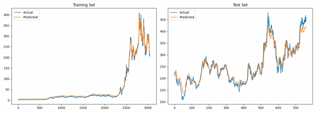
# Visualization
plt.figure(figsize=(14, 5))
plt.subplot(1, 2, 1)
plt.plot(y_train_actual, label='Actual')
plt.plot(train_preds, label='Predicted')
plt.title('Training Set')
plt.legend()
plt.subplot(1, 2, 2)
plt.plot(y_test_actual, label='Actual')
plt.plot(test_preds, label='Predicted')
plt.title('Test Set')
plt.legend()
plt.tight_layout()
plt.show()Predictions align closely with training data, exhibiting typical lag on test set volatility.
Single-Step Forecasting
For one-step-ahead prediction:
last_sequence = scaled_data[-seq_length:].reshape(1, seq_length, 1)
next_pred_scaled = model.predict(last_sequence)
next_pred = scaler.inverse_transform(next_pred_scaled)
print(f"Predicted next day for {stock_symbol}: ${next_pred[0][0]:.2f}")Example output: $235.42 (based on November 2025 data).
Complete Implementation
import numpy as np
import pandas as pd
import yfinance as yf
from sklearn.preprocessing import MinMaxScaler
from tensorflow.keras.models import Model
from tensorflow.keras.layers import Input, LSTM, Dense, Dropout, AdditiveAttention
from tensorflow.keras.optimizers import Adam
import matplotlib.pyplot as plt
import warnings
warnings.filterwarnings('ignore')
# Data fetch
stock_symbol = 'AAPL'
data = yf.download(stock_symbol, start='2010-01-01', end='2025-11-05', auto_adjust=False)
close_prices = data['Close'].values.reshape(-1, 1)
# Preprocessing
scaler = MinMaxScaler(feature_range=(0, 1))
scaled_data = scaler.fit_transform(close_prices)
def create_sequences(data, seq_length):
X, y = [], []
for i in range(len(data) - seq_length):
X.append(data[i:i + seq_length])
y.append(data[i + seq_length])
return np.array(X), np.array(y)
seq_length = 60
X, y = create_sequences(scaled_data, seq_length)
train_size = int(len(X) * 0.8)
X_train, X_test = X[:train_size], X[train_size:]
y_train, y_test = y[:train_size], y[train_size:]
X_train = X_train.reshape((X_train.shape[0], X_train.shape[1], 1))
X_test = X_test.reshape((X_test.shape[0], X_test.shape[1], 1))
# Model
def create_lstm_attention_model(seq_length):
inputs = Input(shape=(seq_length, 1))
x = LSTM(50, return_sequences=True)(inputs)
x = LSTM(50, return_sequences=True)(x)
attention_out = AdditiveAttention()([x, x])
x = LSTM(50, return_sequences=False)(attention_out)
x = Dropout(0.2)(x)
x = Dense(25)(x)
outputs = Dense(1)(x)
model = Model(inputs=inputs, outputs=outputs)
model.compile(optimizer=Adam(learning_rate=0.001), loss='mean_squared_error')
return model
model = create_lstm_attention_model(seq_length)
model.summary()
# Training
history = model.fit(X_train, y_train, epochs=50, batch_size=32,
validation_data=(X_test, y_test), verbose=1)
# Predictions
train_preds = model.predict(X_train)
test_preds = model.predict(X_test)
train_preds = scaler.inverse_transform(train_preds)
y_train_actual = scaler.inverse_transform(y_train.reshape(-1, 1))
test_preds = scaler.inverse_transform(test_preds)
y_test_actual = scaler.inverse_transform(y_test.reshape(-1, 1))
# Plot
plt.figure(figsize=(14, 5))
plt.subplot(1, 2, 1)
plt.plot(y_train_actual, label='Actual')
plt.plot(train_preds, label='Predicted')
plt.title('Training Set')
plt.legend()
plt.subplot(1, 2, 2)
plt.plot(y_test_actual, label='Actual')
plt.plot(test_preds, label='Predicted')
plt.title('Test Set')
plt.legend()
plt.tight_layout()
plt.show()
# Next-day forecast
last_sequence = scaled_data[-seq_length:].reshape(1, seq_length, 1)
next_pred_scaled = model.predict(last_sequence)
next_pred = scaler.inverse_transform(next_pred_scaled)
print(f"Predicted next day for {stock_symbol}: ${next_pred[0][0]:.2f}")Process Terminal:
Model: "functional"
┏━━━━━━━━━━━━━━━━━━━━━┳━━━━━━━━━━━━━━━━━━━┳━━━━━━━━━━━━┳━━━━━━━━━━━━━━━━━━━┓
┃ Layer (type)        ┃ Output Shape      ┃    Param # ┃ Connected to      ┃
┡━━━━━━━━━━━━━━━━━━━━━╇━━━━━━━━━━━━━━━━━━━╇━━━━━━━━━━━━╇━━━━━━━━━━━━━━━━━━━┩
│ input_layer         │ (None, 60, 1)     │          0 │ -                 │
│ (InputLayer)        │                   │            │                   │
├─────────────────────┼───────────────────┼────────────┼───────────────────┤
│ lstm (LSTM)         │ (None, 60, 50)    │     10,400 │ input_layer[0][0] │
├─────────────────────┼───────────────────┼────────────┼───────────────────┤
│ lstm_1 (LSTM)       │ (None, 60, 50)    │     20,200 │ lstm[0][0]        │
├─────────────────────┼───────────────────┼────────────┼───────────────────┤
│ additive_attention  │ (None, 60, 50)    │         50 │ lstm_1[0][0],     │
│ (AdditiveAttention) │                   │            │ lstm_1[0][0]      │
├─────────────────────┼───────────────────┼────────────┼───────────────────┤
│ lstm_2 (LSTM)       │ (None, 50)        │     20,200 │ additive_attenti… │
├─────────────────────┼───────────────────┼────────────┼───────────────────┤
│ dropout (Dropout)   │ (None, 50)        │          0 │ lstm_2[0][0]      │
├─────────────────────┼───────────────────┼────────────┼───────────────────┤
│ dense (Dense)       │ (None, 25)        │      1,275 │ dropout[0][0]     │
├─────────────────────┼───────────────────┼────────────┼───────────────────┤
│ dense_1 (Dense)     │ (None, 1)         │         26 │ dense[0][0]       │
└─────────────────────┴───────────────────┴────────────┴───────────────────┘
 Total params: 52,151 (203.71 KB)
 Trainable params: 52,151 (203.71 KB)
 Non-trainable params: 0 (0.00 B)
Epoch 1/50
99/99 ━━━━━━━━━━━━━━━━━━━━ 6s 44ms/step - loss: 2.4792e-04 - val_loss: 0.0041
Epoch 2/50
99/99 ━━━━━━━━━━━━━━━━━━━━ 4s 43ms/step - loss: 7.2988e-05 - val_loss: 0.0122
Epoch 3/50
99/99 ━━━━━━━━━━━━━━━━━━━━ 4s 43ms/step - loss: 6.3505e-05 - val_loss: 0.0283
Epoch 4/50
99/99 ━━━━━━━━━━━━━━━━━━━━ 4s 44ms/step - loss: 6.8480e-05 - val_loss: 0.0099
Epoch 5/50
99/99 ━━━━━━━━━━━━━━━━━━━━ 4s 44ms/step - loss: 5.3161e-05 - val_loss: 0.0136
Epoch 6/50
99/99 ━━━━━━━━━━━━━━━━━━━━ 4s 43ms/step - loss: 6.0872e-05 - val_loss: 0.0297
Epoch 7/50
99/99 ━━━━━━━━━━━━━━━━━━━━ 4s 44ms/step - loss: 5.4405e-05 - val_loss: 0.0179
Epoch 8/50
99/99 ━━━━━━━━━━━━━━━━━━━━ 4s 44ms/step - loss: 1.0562e-04 - val_loss: 0.0284
Epoch 9/50
99/99 ━━━━━━━━━━━━━━━━━━━━ 4s 44ms/step - loss: 4.9958e-05 - val_loss: 0.0427
Epoch 10/50
99/99 ━━━━━━━━━━━━━━━━━━━━ 4s 43ms/step - loss: 6.6861e-05 - val_loss: 0.0319
Epoch 11/50
99/99 ━━━━━━━━━━━━━━━━━━━━ 4s 44ms/step - loss: 6.1186e-05 - val_loss: 0.0493
Epoch 12/50
99/99 ━━━━━━━━━━━━━━━━━━━━ 5s 46ms/step - loss: 6.1104e-05 - val_loss: 0.0499
Epoch 13/50
99/99 ━━━━━━━━━━━━━━━━━━━━ 4s 44ms/step - loss: 5.5791e-05 - val_loss: 0.0344
Epoch 14/50
99/99 ━━━━━━━━━━━━━━━━━━━━ 4s 44ms/step - loss: 5.6962e-05 - val_loss: 0.0452
Epoch 15/50
99/99 ━━━━━━━━━━━━━━━━━━━━ 4s 44ms/step - loss: 5.6326e-05 - val_loss: 0.0449
Epoch 16/50
99/99 ━━━━━━━━━━━━━━━━━━━━ 4s 44ms/step - loss: 6.8119e-05 - val_loss: 0.0452
Epoch 17/50
99/99 ━━━━━━━━━━━━━━━━━━━━ 4s 44ms/step - loss: 5.2913e-05 - val_loss: 0.0451
Epoch 18/50
99/99 ━━━━━━━━━━━━━━━━━━━━ 4s 44ms/step - loss: 5.1088e-05 - val_loss: 0.0669
Epoch 19/50
99/99 ━━━━━━━━━━━━━━━━━━━━ 4s 43ms/step - loss: 5.9828e-05 - val_loss: 0.0478
Epoch 20/50
99/99 ━━━━━━━━━━━━━━━━━━━━ 4s 43ms/step - loss: 4.9386e-05 - val_loss: 0.0513
Epoch 21/50
99/99 ━━━━━━━━━━━━━━━━━━━━ 4s 44ms/step - loss: 4.8780e-05 - val_loss: 0.0371
Epoch 22/50
99/99 ━━━━━━━━━━━━━━━━━━━━ 4s 45ms/step - loss: 5.8957e-05 - val_loss: 0.0463
Epoch 23/50
99/99 ━━━━━━━━━━━━━━━━━━━━ 5s 45ms/step - loss: 4.8221e-05 - val_loss: 0.0538
Epoch 24/50
99/99 ━━━━━━━━━━━━━━━━━━━━ 5s 48ms/step - loss: 9.2726e-05 - val_loss: 0.0387
Epoch 25/50
99/99 ━━━━━━━━━━━━━━━━━━━━ 5s 47ms/step - loss: 4.3950e-05 - val_loss: 0.0389
Epoch 26/50
99/99 ━━━━━━━━━━━━━━━━━━━━ 5s 48ms/step - loss: 4.4939e-05 - val_loss: 0.0567
Epoch 27/50
99/99 ━━━━━━━━━━━━━━━━━━━━ 5s 49ms/step - loss: 6.1248e-05 - val_loss: 0.0434
Epoch 28/50
99/99 ━━━━━━━━━━━━━━━━━━━━ 5s 47ms/step - loss: 5.3281e-05 - val_loss: 0.0504
Epoch 29/50
99/99 ━━━━━━━━━━━━━━━━━━━━ 4s 44ms/step - loss: 4.9789e-05 - val_loss: 0.0370
Epoch 30/50
99/99 ━━━━━━━━━━━━━━━━━━━━ 4s 44ms/step - loss: 4.2703e-05 - val_loss: 0.0418
Epoch 31/50
99/99 ━━━━━━━━━━━━━━━━━━━━ 4s 44ms/step - loss: 7.4789e-05 - val_loss: 0.0546
Epoch 32/50
99/99 ━━━━━━━━━━━━━━━━━━━━ 4s 44ms/step - loss: 5.2778e-05 - val_loss: 0.0381
Epoch 33/50
99/99 ━━━━━━━━━━━━━━━━━━━━ 4s 44ms/step - loss: 4.5913e-05 - val_loss: 0.0751
Epoch 34/50
99/99 ━━━━━━━━━━━━━━━━━━━━ 4s 44ms/step - loss: 4.6772e-05 - val_loss: 0.0512
Epoch 35/50
99/99 ━━━━━━━━━━━━━━━━━━━━ 4s 45ms/step - loss: 4.4091e-05 - val_loss: 0.0600
Epoch 36/50
99/99 ━━━━━━━━━━━━━━━━━━━━ 4s 45ms/step - loss: 4.1614e-05 - val_loss: 0.0596
Epoch 37/50
99/99 ━━━━━━━━━━━━━━━━━━━━ 4s 44ms/step - loss: 4.1997e-05 - val_loss: 0.0480
Epoch 38/50
99/99 ━━━━━━━━━━━━━━━━━━━━ 4s 44ms/step - loss: 4.6300e-05 - val_loss: 0.0349
Epoch 39/50
99/99 ━━━━━━━━━━━━━━━━━━━━ 4s 45ms/step - loss: 4.8730e-05 - val_loss: 0.0135
Epoch 40/50
99/99 ━━━━━━━━━━━━━━━━━━━━ 4s 45ms/step - loss: 4.0685e-05 - val_loss: 0.0078
Epoch 41/50
99/99 ━━━━━━━━━━━━━━━━━━━━ 5s 46ms/step - loss: 4.9502e-05 - val_loss: 0.0030
Epoch 42/50
99/99 ━━━━━━━━━━━━━━━━━━━━ 4s 44ms/step - loss: 4.9909e-05 - val_loss: 0.0044
Epoch 43/50
99/99 ━━━━━━━━━━━━━━━━━━━━ 4s 44ms/step - loss: 3.1089e-05 - val_loss: 0.0082
Epoch 44/50
99/99 ━━━━━━━━━━━━━━━━━━━━ 4s 44ms/step - loss: 3.1222e-05 - val_loss: 0.0203
Epoch 45/50
99/99 ━━━━━━━━━━━━━━━━━━━━ 5s 46ms/step - loss: 3.5230e-05 - val_loss: 0.0294
Epoch 46/50
99/99 ━━━━━━━━━━━━━━━━━━━━ 4s 44ms/step - loss: 3.5716e-05 - val_loss: 0.0181
Epoch 47/50
99/99 ━━━━━━━━━━━━━━━━━━━━ 4s 45ms/step - loss: 4.7928e-05 - val_loss: 0.0399
Epoch 48/50
99/99 ━━━━━━━━━━━━━━━━━━━━ 4s 44ms/step - loss: 3.1149e-05 - val_loss: 0.0293
Epoch 49/50
99/99 ━━━━━━━━━━━━━━━━━━━━ 4s 44ms/step - loss: 2.6191e-05 - val_loss: 0.0177
Epoch 50/50
99/99 ━━━━━━━━━━━━━━━━━━━━ 4s 44ms/step - loss: 2.9201e-05 - val_loss: 0.0222
99/99 ━━━━━━━━━━━━━━━━━━━━ 1s 13ms/step
25/25 ━━━━━━━━━━━━━━━━━━━━ 0s 11ms/step
Extensions and Considerations
To enhance performance, incorporate additional features (e.g., volume, RSI) or tune hyperparameters via grid search. Monitor for overfitting through validation metrics. For production deployment, integrate with scheduling tools for periodic retraining.
References:
Disclaimer: This model is for illustrative purposes only. Conduct independent verification before any application.