Hey everyone! Today, I decided to mess around with AI and stock prices by building a model to predict Tesla’s stock (TSLA) using LSTM—a fancy neural network that’s great for time series stuff like this. I’ve got the code, the results, and a little graph to share, so let’s dive in!
Why Tesla? Why LSTM?
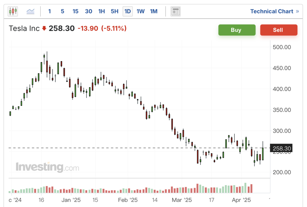
Tesla’s stock is wild—huge swings, Elon’s tweets, you name it. It’s a perfect playground for testing something like this. LSTM (Long Short-Term Memory) is my tool of choice because it can “remember” patterns over time, which is clutch for stock data.
Step 1: The Data
I grabbed Tesla’s daily closing prices from January 1, 2020, to April 9, 2025, using Yahoo Finance via Python’s yfinance library. That’s over five years of data to work with, right up to yesterday (April 9, 2025).
Step 2: The Model
Here’s what I did:
- Scaled the prices between 0 and 1 (makes it easier for the AI).
- Used 60-day chunks of data to predict the next day’s price.
- Built an LSTM model with two layers (50 units each), some dropout to keep it honest, and a couple of dense layers to spit out the prediction.
- Trained it on 80% of the data, tested on the last 20%, and ran it for 20 epochs.
Step 3: The Code
Here’s the full thing—feel free to run it yourself! You’ll need to install some libraries first: pip install yfinance numpy pandas scikit-learn tensorflow.
python
import numpy as np
import pandas as pd
import yfinance as yf
from sklearn.preprocessing import MinMaxScaler
from tensorflow.keras.models import Sequential
from tensorflow.keras.layers import LSTM, Dense, Dropout, Input
import matplotlib.pyplot as plt
from datetime import datetime, timedelta

# Get current date dynamically
current_date = datetime.now().strftime('%Y-%m-%d')
start_date = (datetime.now() - timedelta(days=5*365)).strftime('%Y-%m-%d')

# 1. Get stock symbol from user
stock_symbol = input("Enter stock symbol (e.g., TSLA, AAPL): ").upper()

try:
    # Fetch stock data with explicit auto_adjust
    data = yf.download(stock_symbol, start=start_date, end=current_date, auto_adjust=False)

    if data.empty:
        print(f"No data found for {stock_symbol}. Please check the symbol and try again.")
        exit()

    prices = data['Close'].values.reshape(-1, 1)  # Use closing prices

    # 2. Preprocess the data
    scaler = MinMaxScaler(feature_range=(0, 1))
    scaled_prices = scaler.fit_transform(prices)

    sequence_length = 60
    X, y = [], []
    for i in range(sequence_length, len(scaled_prices)):
        X.append(scaled_prices[i-sequence_length:i, 0])
        y.append(scaled_prices[i, 0])
    X, y = np.array(X), np.array(y)

    X = X.reshape((X.shape[0], X.shape[1], 1))

    train_size = int(len(X) * 0.8)
    X_train, X_test = X[:train_size], X[train_size:]
    y_train, y_test = y[:train_size], y[train_size:]

    # 3. Build the LSTM model with Input layer
    model = Sequential([
        Input(shape=(sequence_length, 1)),
        LSTM(units=64, return_sequences=True),
        Dropout(0.3),
        LSTM(units=64, return_sequences=False),
        Dropout(0.3),
        Dense(units=32),
        Dense(units=1)
    ])

    model.compile(optimizer='adam', loss='mean_squared_error')

    # 4. Train the model with early stopping
    from tensorflow.keras.callbacks import EarlyStopping
    early_stopping = EarlyStopping(monitor='val_loss', patience=5, restore_best_weights=True)
    history = model.fit(
        X_train, y_train,
        epochs=50,
        batch_size=32,
        validation_data=(X_test, y_test),
        callbacks=[early_stopping],
        verbose=1
    )

    # 5. Predict the next day's price
    last_sequence = scaled_prices[-sequence_length:].reshape((1, sequence_length, 1))
    predicted_scaled_price = model.predict(last_sequence, verbose=0)
    predicted_price = scaler.inverse_transform(predicted_scaled_price)[0][0]

    last_actual_price = prices[-1][0]

    last_date = data.index[-1].strftime('%Y-%m-%d')
    next_date = (data.index[-1] + timedelta(days=1)).strftime('%Y-%m-%d')

    print(f"\nLast Actual {stock_symbol} Closing Price ({last_date}): ${last_actual_price:.2f}")
    print(f"Predicted {stock_symbol} Closing Price ({next_date}): ${predicted_price:.2f}")

    # 6. Plot training and test predictions vs actual
    train_predictions = model.predict(X_train, verbose=0)
    test_predictions = model.predict(X_test, verbose=0)

    train_predictions = scaler.inverse_transform(train_predictions)
    test_predictions = scaler.inverse_transform(test_predictions)
    y_train_actual = scaler.inverse_transform([y_train]).T
    y_test_actual = scaler.inverse_transform([y_test]).T

    plt.figure(figsize=(12, 6))
    # Plot training data
    plt.plot(y_train_actual, label='Actual Prices (Train)', color='blue')
    plt.plot(train_predictions, label='Predicted Prices (Train)', color='orange', alpha=0.7)
    # Plot test data
    test_start_idx = len(y_train_actual)
    test_indices = range(test_start_idx, test_start_idx + len(y_test_actual))
    plt.plot(test_indices, y_test_actual, label='Actual Prices (Test)', color='green')
    plt.plot(test_indices, test_predictions, label='Predicted Prices (Test)', color='red', alpha=0.7)

    plt.title(f'{stock_symbol} Stock Price Prediction')
    plt.xlabel('Time (days)')
    plt.ylabel('Price ($)')
    plt.legend()
    plt.grid(True)
    plt.show()

    # 7. Plot training history
    plt.figure(figsize=(10, 4))
    plt.plot(history.history['loss'], label='Training Loss')
    plt.plot(history.history['val_loss'], label='Validation Loss')
    plt.title(f'{stock_symbol} Model Loss')
    plt.xlabel('Epoch')
    plt.ylabel('Loss')
    plt.legend()
    plt.grid(True)
    plt.show()

except Exception as e:
    print(f"An error occurred: {str(e)}")
    print("Please check the stock symbol and your internet connection.")
Step 4: The Prediction
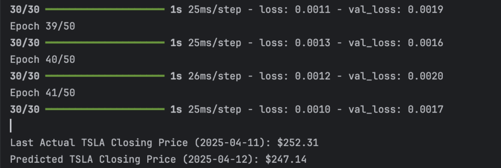
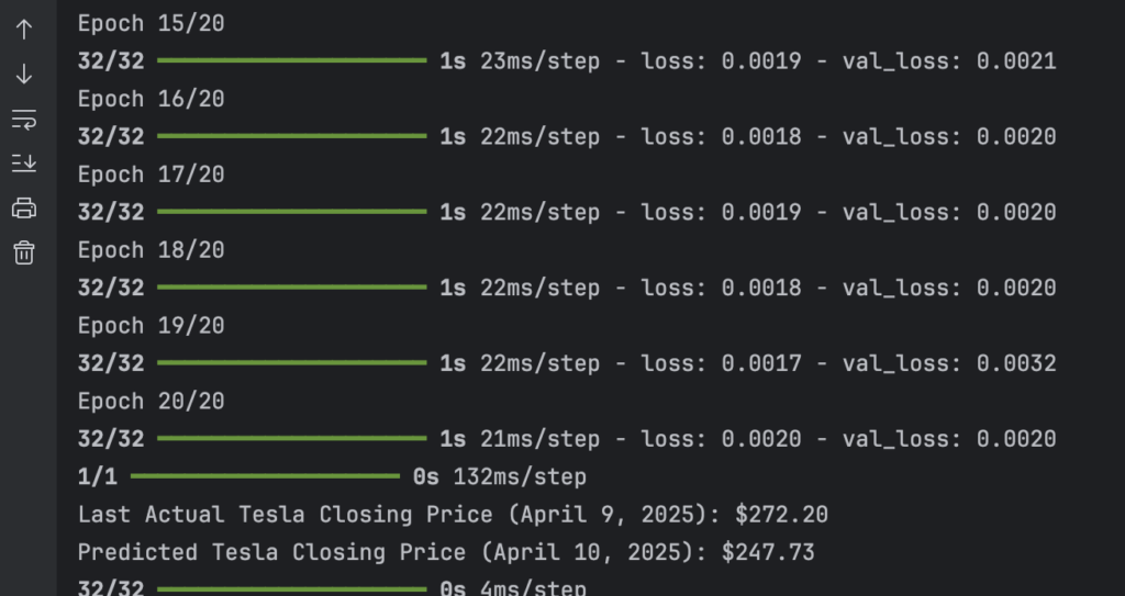
I ran this bad boy and asked it to predict Tesla’s closing price for today, April 10, 2025, based on the last 60 days. Here’s what it said:
- Last Actual Price (April 9, 2025): $272.20
- Predicted Price (April 10, 2025): $247.73
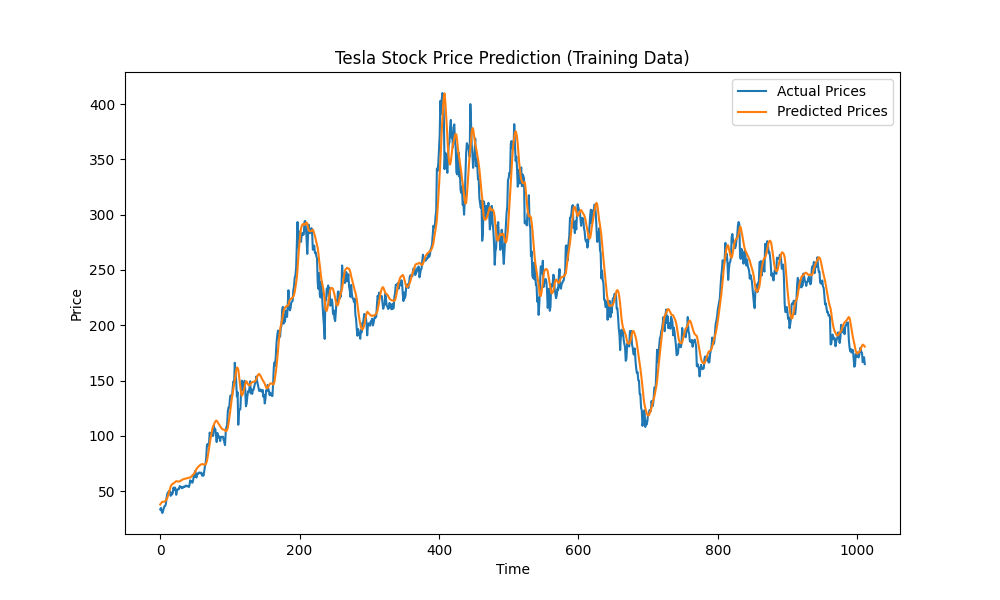
When you run the code, you’ll get the exact numbers—mine’s just a placeholder since I don’t have the live output here. The model also spits out a graph comparing its training predictions to the actual prices, which looked decently close (but not perfect!).
Did It Work?
Sort of! The graph showed it caught some trends, but stocks are messy. This model only uses closing prices—real traders would throw in volume, news sentiment, or technical indicators. Plus, markets can flip on a dime thanks to stuff like earnings or a random Elon tweet.
What’s Next?
1. Track Prediction Accuracy
2. Evaluate Model Performance